Saturday, September 21, 2019

Python NdArray

Ndarray:

The most important object defined in NumPy is an N-dimensional array type called ndarray. It describes the collection of items of the same type. Items in the collection can be accessed using a zero-based index.

The ndarray object consists of contiguous one-dimensional segment of computer memory, combined with an indexing scheme that maps each item to a location in the memory block. The memory block holds the elements in a row-major order (C style) or a column-major order (FORTRAN or MatLab style).

Creation:

numpy.array(object,

                                       dtype = None,

                                       copy = True,

                                       order = None,

                                       ndmin = 0)

Object : Any object exposing the array interface method returns an array, or any (nested) sequence.

Dtype :Desired data type of array, optional

Copy: Optional. By default (true), the object is copied

Order: C (row major) or F (column major) or A (any) (default)

Ndmin: Specifies minimum dimensions of resultant array

Attributes:

ndarray.ndim: The number of axes (dimensions) of the array.

ndarray.shape: The dimensions of the array. This is a tuple of integers indicating the size of the array in each dimension. For a matrix with nrows and m columns, shape will be (n,m). The length of the shape tuple is therefore the number of axes, ndim.

ndarray.size: The total number of elements of the array. This is equal to the product of the elements of shape.

ndarray.dtype: An object describing the type of the elements in the array. One can create or specify dtype’s using standard Python types. Additionally, NumPy provides types of its own. numpy.int32, numpy.int16, and numpy.float64 are some examples.

ndarray.itemsize: The size in bytes of each element of the array. For example, an array of elements of type float64 has itemsize 8 (=64/8), while one of type complex32 has itemsize 4 (=32/8). It is equivalent to ndarray.dtype.itemsize.

ndarray.data: tTe buffer containing the actual elements of the array. Normally, we won’t need to use this attribute because we will access the elements in an array using indexing facilities.

Data Types:

The following examples define a structured data type called student with a string field 'name', an integer field 'age' and a float field 'marks'. This dtype is applied to ndarray object.

Import numpy as np

dt = np.dtype(np.int32)

Student = np.dtype([('name','S20'), ('age', 'i1'), ('marks', 'f4')])

print student

Each built-in data type has a character code that uniquely identifies it


Python numPy Array functions

Python numPy:
NumPy is the core library for scientific computing in python. It provides a high-performance multidimensional array object, and tools for working with these arrays. Numpy can also be used as an efficient multi-dimensional container of generic data. Moreover, it is fast and reliable. Numpy functions return either views or copies.

Python numpy Array:
NumPy arrays are a bit like Python lists, but still very much different at the same time. A NumPy array is a central data structure of the numpy library ("Numeric Python" or "Numerical Python").


Create a numPy Array:
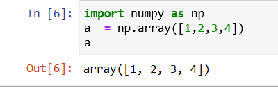
Simplest way to create an array in numpy is to use Python List


Or 


Mathematical Operations on an Array:


Shape and dtype of Array:

Shape: is the shape of the array

Dtype: is the datatype. It is optional. The default value is float64


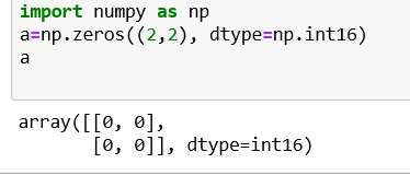
np.zeros and np.ones:
You can create a matrix full of zeroes or ones using np.zeros and np.one commands respectively. It can be used when you initialized the weights during the first iteration in TensorFlow and other statistic tasks.


The syntax is:
numpy.zeros(shape, dtype=float, order='C')


numpy.ones(shape, dtype=float, order='C')


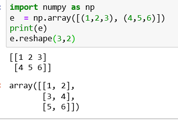
numpy.reshape() and numpy.flatten() : 

Reshape Data: In some occasions, you need to reshape the data from wide to long. You can use the reshape function for this.

The syntax is
numpy.reshape(a, newShape, order='C')

Here,

a: Array that you want to reshape

newShape: The new desires shape

Order: Default is C which is an essential row style.


Flatten Data: When you deal with some neural network like convnet, you need to flatten the array. You can use flatten().

The syntax is
numpy.flatten(order='C')

Here,

Order: Default is C which is an essential row style.


numpy.hstack() and numpy.vstack():


With hstack you can appended data horizontally. This is a very convenient function in Numpy. 


With vstack you can appened data vertically.


Generate Random Numbers: To generate random numbers for Gaussian distribution use
numpy.random.normal(loc, scale, size)
Here,

Loc: the mean. The center of distribution

scale: standard deviation.

Size: number of returns


numpy.asarray() :
The asarray() function is used when you want to convert an input to an array. The input could be a lists, tuple, ndarray, etc.
Syntax:

numpy.asarray(data, dtype=None, order=None)[source]

Here,

data: Data that you want to convert to an array

dtype: This is an optional argument. If not specified, the data type is inferred from the input data

Order: Default is C which is an essential row style. Other option is F (Fortan-style)


Matrix is immutable. You can use asarray if you want to add modification in the original array. 


Example:

If you want to change the value of the third rows with the value 2np.

asarray(A): converts the matrix A to an array

[2]: select the third rows


numpy.arange() :

Sometimes, you want to create values that are evenly spaced within a defined interval. For instance, you want to create values from 1 to 10; you can use numpy.arange() function.

Syntax:

numpy.arange(start, stop,step) 

Here,

Start: Start of interval

Stop: End of interval

Step: Spacing between values. Default step is 1


numpy.linspace() and numpy.logspace():
Linspace: Linspace gives evenly spaced samples.


Syntax:

numpy.linspace(start, stop, num, endpoint)

Here,

Start: Starting value of the sequence

Stop: End value of the sequence

Num: Number of samples to generate. Default is 50

Endpoint: If True (default), stop is the last value. If False, stop value is not included.


If you do not want to include the last digit in the interval, you can set endpoint to false
np.linspace(1.0, 5.0, num=5, endpoint=False)


LogSpace: LogSpace returns even spaced numbers on a log scale. Logspace has the same parameters as np.linspace.


Syntax:
numpy.logspace(start, stop, num, endpoint)


Finally, if you want to check the size of an array, you can use itemsize


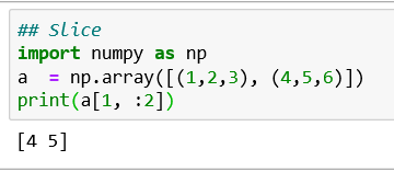
Indexing and Slicing NumPy Arrays:
Slicing data is trivial with numpy. We will slice the matrices "e". Note that, in Python, you need to use the brackets to return the rows or columns


Note: The values before the comma stand for the row. The value on the rights stands for the columns. If you want to select a column, you need to add: before the column index.: means you want all the rows from the selected column.


To return the first two values of the second row. You use: to select all columns up to the second


NumPy Statistical Functions:
NumPy has quite a few useful statistical functions for finding minimum, maximum, percentile standard deviation and variance, etc from the given elements in the array.


numpy.dot():
Dot Product: Numpy is powerful library for matrices computation. For instance, you can compute the dot product with np.dot
Syntax:

numpy.dot(x, y, out=None)

Here,

x,y: Input arrays. x and y both should be 1-D or 2-D for the function to work

out: This is the output argument. For 1-D array scalar is returned. Otherwise ndarray.


NumPy Matrix Multiplication with np.matmul() :
The Numpu matmul() function is used to return the matrix product of 2 arrays. Here is how it works1) 2-D arrays, it returns normal product2) Dimensions > 2, the product is treated as a stack of matrix3) 1-D array is first promoted to a matrix, and then the product is calculated
numpy.matmul(x, y, out=None)

Here,

x,y: Input arrays. scalars not allowed
out: This is optional parameter. Usually output is stored in ndarray


Determinant:
Last but not least, if you need to compute the determinant, you can use np.linalg.det(). Note that numpy takes care of the dimension.


Importing and Exporting Of Files:

import numpy as np

np.loadtxt (file.txt)   # imports from a text file

np.savetxt (‘file.txt’,arr,delimiter= ’  ’)   #writes to a text file


Wednesday, September 18, 2019

T-Test VS Z-Test Comparison

Hypothesis Test (t-test Vs z-test):

Hypothesis:  A supposition which must be accepted or rejected is called as a hypothesis.

 Hypothesis testing procedures are classified in to 2 types:

  1) Parametric test (Is based on the fact, that the variables are measured on an interval scale)

a) t-test

b) z-test

  2) Non-parametric test (Is assumed to be measured on an ordinal scale)           

T-Test and Z-test Comparison:


T-Test

Z-Test

Definition:

T-test refers to a univariate hypothesis test based on t-statistic, wherein the mean is known, and population variance is approximated from the sample.

è More precisely, a t-test is used to examine how the means taken from two independent samples differ.

è T-test follows t-distribution, which is appropriate when the sample size is small, and the population standard deviation is not known.

è The shape of a t-distribution is highly affected by the degree of freedom. The degree of freedom implies the number of independent observations in a given set of observations.


Paired t-test: A statistical test applied when the two samples are dependent and paired observations are taken.


Z-test is also a univariate test that is based on standard normal distribution.


è Z-test refers to a univariate statistical analysis used to test the hypothesis that proportions from two independent samples differ greatly.

è It determines to what extent a data point is away from its mean of the data set, in standard deviation.

è Z-test can be adopted when the population variance is known when there is a large sample size, sample variance is deemed to be approximately equal to the population variance.

Key Differences:

è Based on t-distribution.

è T-test can be applied when the means of the two population is different from one another.

è Population variance is unknown.

è Can be applied when Sample Size is Small (<30)

è Based on Normal-distribution.

è Z-test can be applied when the standard deviation is known, to determine, if the means of the two datasets differ from each other.

è Population variance is known.

è Can be applied when Sample Size is large (>30)

Assumptions:

  • All data points are independent.
  • The sample size is small. Generally, a sample size exceeding 30 sample units is regarded as large, otherwise small but that should not be less than 5, to apply t-test.
  • Sample values are to be taken and recorded accurately.

The test statistic is:


x ̅is the sample mean
s is sample standard deviation
n is sample size and μ is the population mean

  • All sample observations are independent
  • Sample size should be more than 30.
  • Distribution of Z is normal, with a mean zero and variance 1.


The test statistic is:


x ̅is the sample mean
σ is population standard deviation
n is sample size
μ is the population mean


Useful Flow Charts:


Examples:

Z-Test Example:

 Suppose, the mean height of women is 65″ with a standard deviation of 3.5″. What is the probability of finding a random sample of 50 women with a mean height of 70″, assuming the heights are normally distributed?

  z = (x – μ) / (σ / √n)   =  (70 – 65) / (3.5/√50) = 5 / 0.495 = 10.1

 The key here is that we’re dealing with a sampling distribution of means, so we know we have to include the standard error in the formula.

 We also know that 99% of values fall within 3 standard deviations from the mean in a normal probability distribution.

 Therefore, there’s less than 1% probability that any sample of women will have a mean height of 70″.

Example for Independent t-test:

 A research study was conducted to examine the differences between older and younger adults on perceived life satisfaction. A pilot study was conducted to examine this hypothesis. Ten older adults (over the age of 70) and ten younger adults (between 20 and 30) were give a life satisfaction test (known to have high reliability and validity). Scores on the measure range from 0 to 60 with high scores indicative of high life satisfaction; low scores indicative of low life satisfaction. The data are presented below.

Older Adults                                                                                                     Younger Adults

               45                                                                                                                    34

               38                                                                                                                    22

               52                                                                                                                    15

               48                                                                                                                    27

               25                                                                                                                    37

               39                                                                                                                    41

               51                                                                                                                    24

               46                                                                                                                    19

               55                                                                                                                    26

               46                                                                                                                    36

 Mean = 44.5                                                                                                 Mean = 28.1,

S = 8.682677518                                                                                          S = 8.543353492

S2 = 75.388888888                                                                                        S2 = 72.988888888                                                  

By using the formula for t-test, the appropriate t-test value is = 4.257


Saturday, September 14, 2019

Bayes' Theorem

Bayes’ Theorem:

 Bayes’ Theorem is a way of finding a Probability when we know certain other probabilities.

The formula is: P(A|B) = P(A) P(B|A) / P(B)

Where

P(B|A)=How often B happens given that A happens

P(A|B)= How often A happens given that B happens

P(A) = How likely A is on its own

P(B) = How likely B is on its own

Description:

Let {E1,E2,…,En} be a set of events associated with a sample space S, where all the events E1,E2,…,En have nonzero probability of occurrence and they form a partition of S. Let A be any event associated with S, then according to Bayes theorem,

Explanation:

According to conditional probability formula,

Using multiplication rule of probability,                   


Using total probability theorem,


From equations 2 and 3:

Descriptive Statistics

Descriptive Statistics:         

Central Tendency (or Groups’ “Middle Values”)

       Mean, Median, Mode

Variation (or Summary of Differences Within Groups)

     Range, Interquartile Range, Variance, Standard Deviation

Mean:

  • Most commonly called the “average.”
  • Add up the values for each case and divide by the total number of cases.
  • Means can be badly affected by outliers (data points with extreme values unlike the rest)
  • Outliers can make the mean a bad measure of central tendency or common experience

Y-bar  =    (Y1 + Y2 + . . . + Yn) / n  OR   Y-bar  =   Σ Yi/ n

Example:

Mean of below numbers              

102,115,128,109,131,89,98,106  ,140,119,93,97,110

Σ Yi = 102+115+128+109+131+89+98+106+140+119+93+97+110=1437

Y-barA  =   Σ Yi = 1437/13 = 110.54     

Median:

  • The middle value when a variable’s values are ranked in order; the point that divides a distribution into two equal halves.
  • When data are listed in order, the median is the point at which 50% of the cases are above and 50% below it.
  • The 50th
  • The median is unaffected by outliers, making it a better measure of central tendency, better describing the “typical person” than the mean when data are skewed.
  • If the recorded values for a variable form a symmetric distribution, the median and mean are identical.
  • In skewed data, the mean lies further toward the skew than the median.

Example:

Consider below numbers:            

89,93,97,98,102,106,109,110,115,119,128,131,140          

Mode:

  • The most common data point is called the mode.
  • It is possible to have more than one mode.
  • It may give you the most likely experience rather than the “typical” or “central” experience.
  • In symmetric distributions, the mean, median, and mode are the same.
  • In skewed data, the mean and median lie further toward the skew than the mode.

Consider below numbers:

80 87 89 93 93 96 97 98 102 103 105 106 109 109 109 110 111 115 119 120 127 128 131 131 140 162

Range:

  • The spread, or the distance, between the lowest and highest values of a variable.
  • To get the range for a variable, you subtract its lowest value from its highest value.

Example:

102,115,128,109,131,89,98,106,140,119,93,97,110

Range = 140 - 89 = 51

Interquartile Range:

  • A quartile is the value that marks one of the divisions that breaks a series of values into four equal parts.
  • The median is a quartile and divides the cases in half.
  • 25th percentile is a quartile that divides the first ¼ of cases from the latter ¾.
  • 75th percentile is a quartile that divides the first ¾ of cases from the latter ¼.

Variance:

  • A measure of the spread of the recorded values on a variable. A measure of dispersion.
  • The larger the variance, the further the individual cases are from the mean.
  • The smaller the variance, the closer the individual scores are to the mean.
  • Variance is a number that at first seems complex to calculate.
  • Calculating variance starts with a “deviation.”
  • A deviation is the distance away from the mean of a case’s score.

Variance = Σ(Yi – Y-bar)2 / n – 1

Standard Deviation:

  • To convert variance into something, create standard deviation.
  • The square root of the variance reveals the average deviation of the observations from the mean.

S.D.  = Square root  ( Σ(Yi – Y-bar)2  /(n-1) )                       

The Central Limit Theorem

The central limit theorem:

  • Mean is μ
  • Standard deviation σ
  • Consider large random samples from the population (Repetition is Allowed) and sample size is sufficiently large (n >30) 

Then the distribution of the sample means will be approximately normally distributed. This will hold true regardless of whether the source population is normal or skewed.

The formula for central limit theorem can be stated as follows:

and

Where:


μ       =  Population mean
σ       =  Population standard deviation
μx¯   =  Sample mean
σx¯   =  Sample standard deviation
n      =  Sample size 


ML-Model DecisionTree Example-IncomePrediction

DecisionTree -- IncomePrediction Decision Tree: Income Prediction ¶ In this l...